Cytoscape Automation in R using Rcy3
Ruth Isserlin
July 26, 2018
BioC 2018 - Toronto, Ontario

Overview
- Ruth Isserlin - ruth dot isserlin (at) utoronto (dot) ca
- Brendan Innes - brendan (dot) innes (at) mail (dot) utoronto (dot) ca
- Jeff Wong - jvwong (at) gmail (dot) com
- Gary Bader - gary (dot) bader (at) utoronto (dot) ca
Download and Install:
- Slides - https://cytoscape.github.io/cytoscape-tutorials/presentations/bioc2018_Rcy3_intro#/
- Cytoscape - http://www.cytoscape.org/download.php
- RNotebook files - https://github.com/Bioconductor/BiocWorkshops/blob/master/230_Isserlin_RCy3_intro.Rmd
- Workshop Book - https://bioconductor.github.io/BiocWorkshops/BioC2018.pdf
- R packages (list below)
- Cytoscape Apps (listed below) - in Cytoscape go to Apps->App Manager to install apps.
| in RStudio install the following packages |
|---|
| RCy3 |
| gProfileR |
| RCurl |
| EnrichmentBrowser |
| in Cytoscape install |
|---|
| EnrichmentMap pipeline Collection |
| Functional Enrichment Collection |
| aMatReader |
Prerequisites
| Workshop prerequisites |
|---|
| Basic knowledge of R syntax |
| Basic knowledge of Cytoscape software |
| Familiarity with network biology concepts |
| R / Bioconductor packages |
|---|
| RCy3 |
| gProfileR |
| RCurl |
| EnrichmentBrowser |
Outline
| Activity | Time |
|---|---|
| Introduction | 15m |
| Driving Cytoscape from R | 15m |
| Creating, retrieving and manipulating networks | 15m |
| Summary | 10m |
Workshop goals and objectives
Learning goals - Know when and how to use Cytoscape in your research area
- Generalize network analysis methods to multiple problem domains
- Integrate Cytoscape into your bioinformatics pipelines
Learning objectives - Programmatic control over Cytoscape from R
- Publish, share and export networks
Background
Cytoscape

- Cytoscape(Shannon et al.) is a freely available open-source, cross platform network analysis software.
- Cytoscape(Shannon et al.) can visualize complex networks and help integrate them with any other data type.
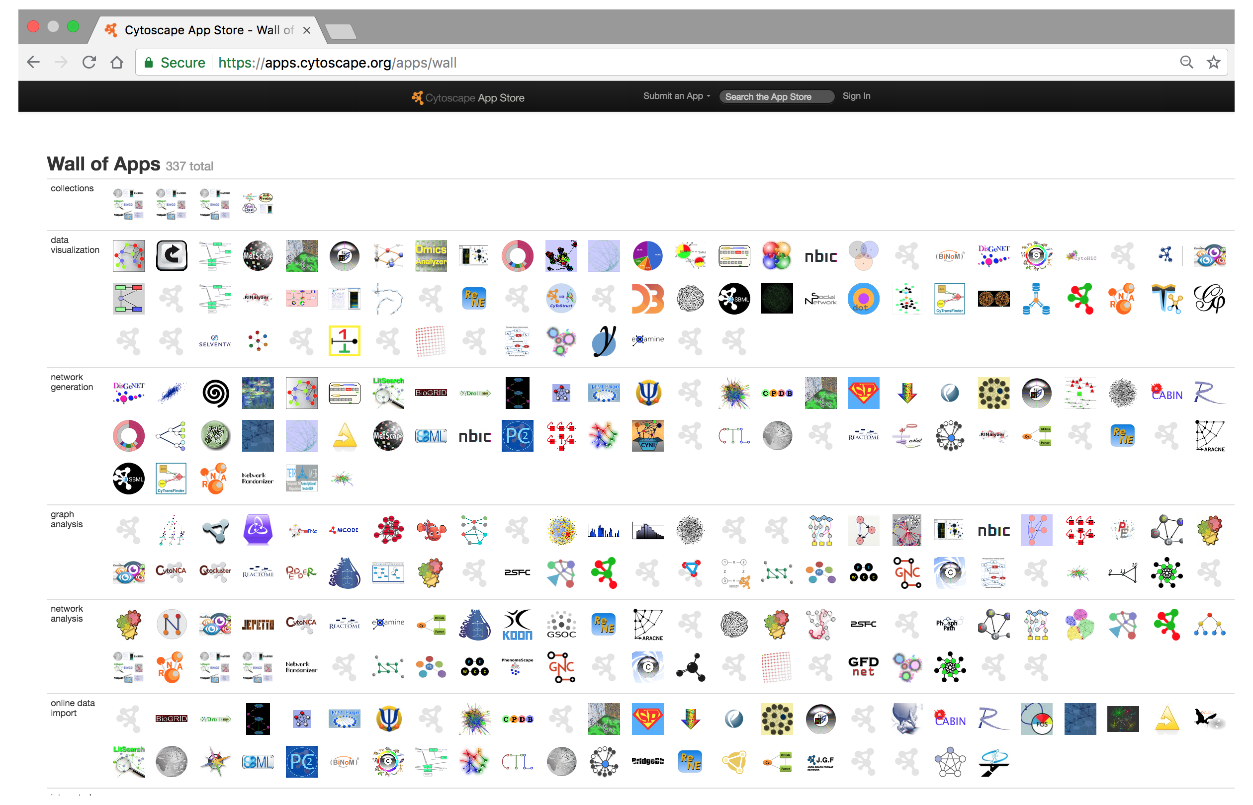
- Cytoscape(Shannon et al.) has an active developer and user base with more than 300 community created apps available from the (Cytoscape App Store)[apps.cytoscape.org].
- Check out some of the tasks you can do with Cytoscape in our online tutorial guide - tutorials.cytoscape.org
Cytoscape Apps
Overview of network biology themes and concepts
Why Networks?
Networks are everywhere… - Molecular Networks
- Cell-Cell communication Networks
- Computer networks
- Social Networks
- Internet
Networks are powerful tools… - Reduce complexity
- More efficient than tables
- Great for data integration
- Intuitive visualization
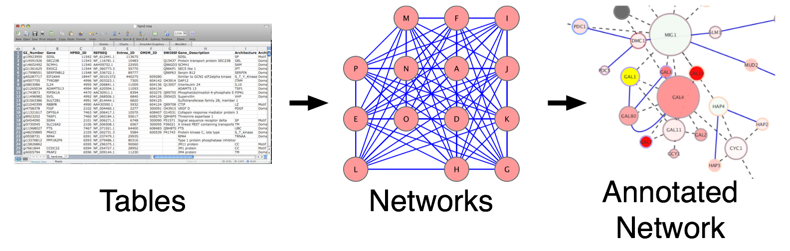
Often data in our pipelines are represented as data.frames, tables, matrices, vectors or lists. Sometimes we represent this data as heatmaps, or plots in efforts to summarize the results visually. Network visualization offers an additional method that readily incorporates many different data types and variables into a single picture.
Network types
Networks as Tools
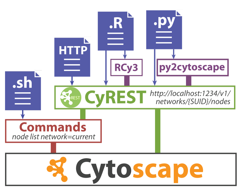
Translating biological data into Cytoscape using RCy3
Networks offer us a useful way to represent our biological data. But how do we seamlessly translate our data from R into Cytoscape?
Set up
Set up - (part 2)
Set up - (part 4)
Communicating with Cytoscape
Make sure that Cytoscape is open
cytoscapePing ()

Getting started
Confirm that Cytoscape is installed and opened
cytoscapeVersionInfo ()

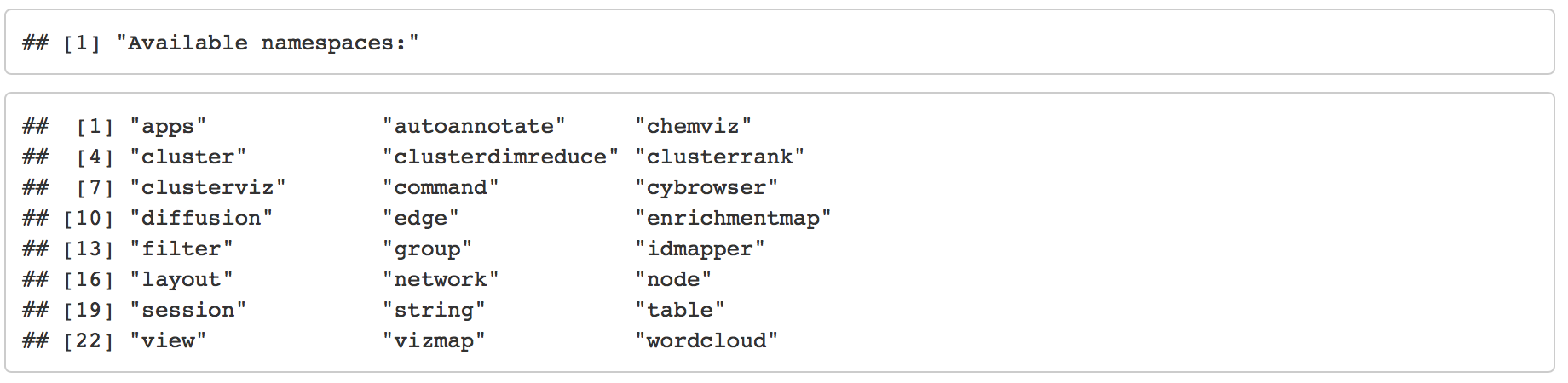
Browse available functions, commands and arguments
Help on specific cytoscape command
To get information about an individual command from the R environment you can also use the commandsHelp function. Simply specify what command you would like to get information on by adding its name to the command. For example “commandsHelp("help string”)“
commandsHelp("help")
Cytoscape Basics
Data frame used to create Network
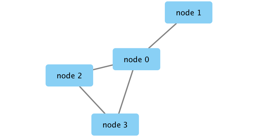
Create Network
createNetworkFromDataFrames(nodes,edges, title="my first network", collection="DataFrame Example")
Export an image of the network
Initial simple network
Example Data Set
There are two data files:
- Expression matrix - containing the normalized expression for each gene across all 300 samples.
- Gene ranks - containing the p-values, FDR and foldchange values for the 4 comparisons (mesenchymal vs rest, differential vs rest, proliferative vs rest and immunoreactive vs rest)
RNASeq_expression_matrix <- read.table(
                          file.path(getwd(),"230_Isserlin_RCy3_intro","data","TCGA_OV_RNAseq_expression.txt"),
                          header = TRUE, sep = "\t", quote="\"", stringsAsFactors = FALSE)

RNASeq_gene_scores <- read.table(
                           file.path(getwd(),"230_Isserlin_RCy3_intro","data","TCGA_OV_RNAseq_All_edgeR_scores.txt"),
                          header = TRUE, sep = "\t", quote="\"", stringsAsFactors = FALSE)
Finding Network Data
Use Case 1 - How are my top genes related?
Omics data - I have a -----------fill in the blank (microarray, RNASeq, Proteomics, ATACseq, MicroRNA, GWAS …) dataset. I have normalized and scored my data. How do I overlay my data on existing interaction data?
There are endless amounts of databases storing interaction data.
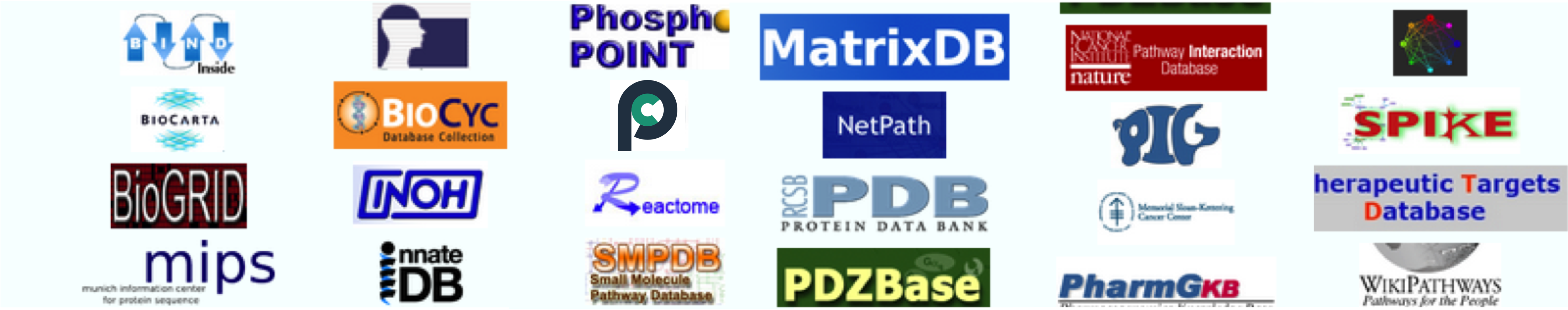
Cytoscape Apps with network data
commandsHelp("help string")
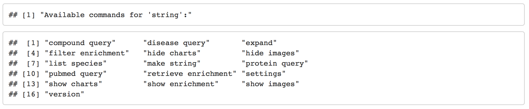
commandsHelp("help string protein query")
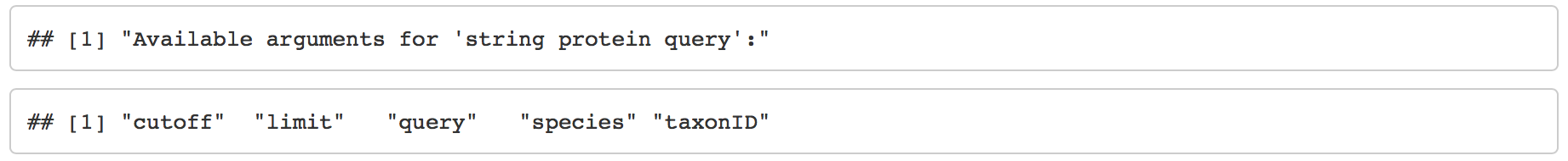
Query String
mesen_string_interaction_cmd <- paste('string protein query taxonID=9606 limit=150 cutoff=0.9 query="',paste(top_mesenchymal_genes$Name, collapse=","),'"',sep="")
commandsGET(mesen_string_interaction_cmd)

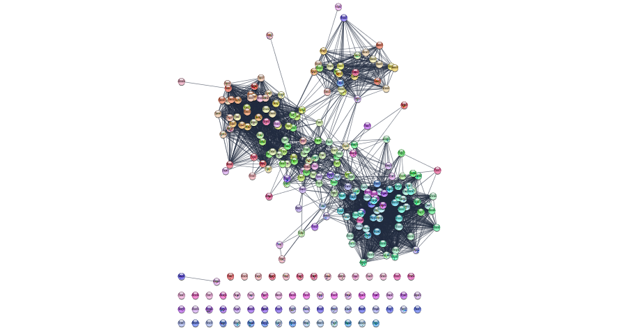
Initial String Network - top Mesenchymal genes interactions
Layouts
Layout the network
layoutNetwork('force-directed')
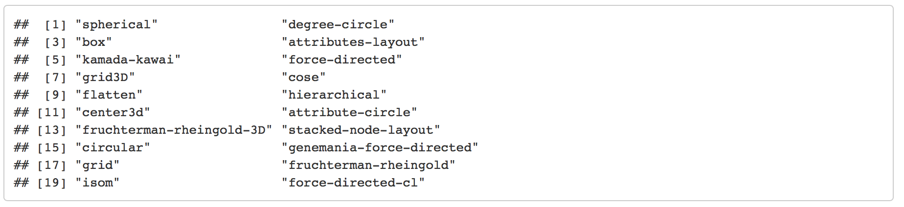
Check what other layout algorithms are available to try out
getLayoutNames()
Layouts - cont'd
Get the parameters for a specific layout
getLayoutPropertyNames(layout.name='force-directed')

Layouts - cont'd
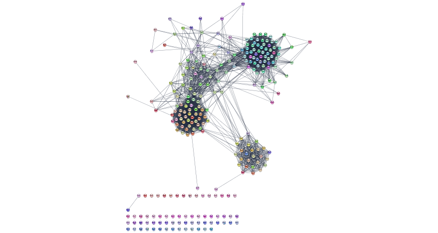
String network with new layout
Overlay our expression data on the String network.
To do this we will be using the loadTableData function from RCy3. It is important to make sure that that your identifiers types match up. You can check what is used by String by pulling in the column names of the node attribute table.
getTableColumnNames('node')
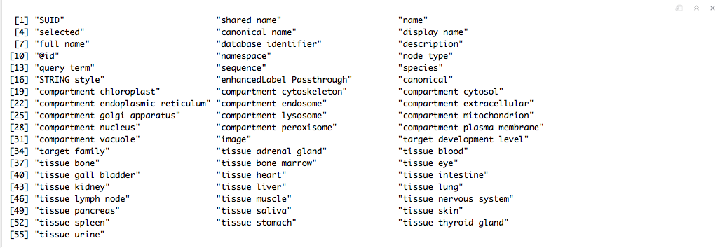
Overlay our expression data on the String network - cont'd
If you are unsure of what each column is and want to further verify the column to use you can also pull in the entire node attribute table.
node_attribute_table_topmesen <- getTableColumns(table="node")
head(node_attribute_table_topmesen[,3:7])
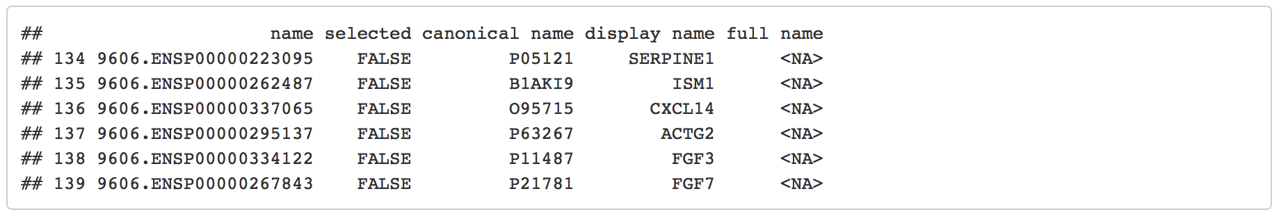
Overlay our expression data on the String network - cont'd
The column “display name” contains HGNC gene names which are also found in our Ovarian Cancer dataset.
To import our expression data we will match our dataset to the “display name” node attribute.
?loadTableData

loadTableData(RNASeq_gene_scores,table.key.column = "display name",
data.key.column = "Name")  #default data.frame key is row.names

Visual Style
Modify the visual style Create your own visual style to visualize your expression data on the String network.
Start with a default style
style.name = "MesenchymalStyle"
defaults.list <- list(NODE_SHAPE="ellipse",
                 NODE_SIZE=60,
                 NODE_FILL_COLOR="#AAAAAA",
                 EDGE_TRANSPARENCY=120)
# p for passthrough; nothing else needed
node.label.map <- mapVisualProperty('node label','display name','p')
createVisualStyle(style.name, defaults.list, list(node.label.map))
setVisualStyle(style.name=style.name)

Visual Style - cont'd
Visual Style - cont'd
Next, we use the RColorBrewer package to help us pick good colors to pair with our data values.
library(RColorBrewer)
display.brewer.all(length(data.values), colorblindFriendly=TRUE, type="div")

logFC to node color
node.colors <- c(rev(brewer.pal(length(data.values), "RdBu")))
Map the colors to our data value and update our visual style.
setNodeColorMapping("logFC.mesen", data.values, node.colors, style.name=style.name)
Visual Style - cont'd
Remember, String includes your query proteins as well as other proteins that associate with your query proteins (including the strongest connection first). Not all of the proteins in this network are your top hits. How can we visualize which proteins are our top Mesenchymal hits?
Add a different border color or change the node shape for our top hits.
getNodeShapes()

#select the Nodes of interest
#selectNode(nodes = top_mesenchymal_genes$Name, by.col="display name")
setNodeShapeBypass(node.names = top_mesenchymal_genes$Name, new.shapes = "TRIANGLE")

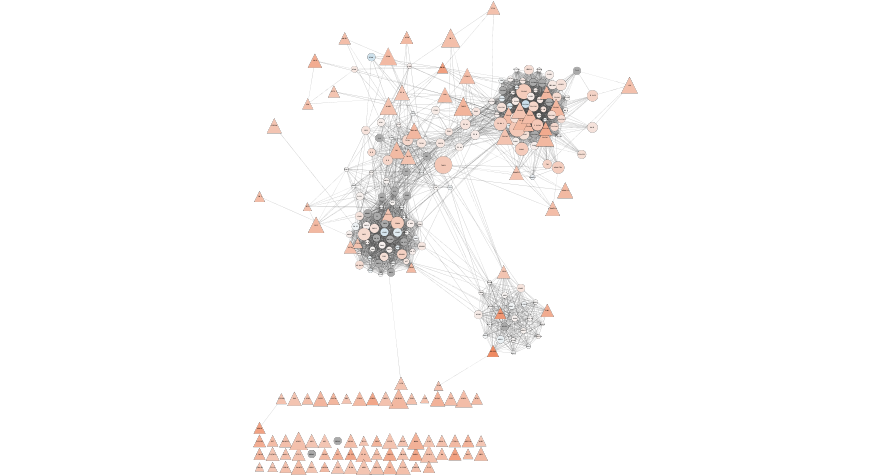
Visual Style - cont'd
Visual Style - cont'd
Formatted String network
Use Case 2 - Which genes have similar expression.
Use the CyRest call to access the aMatReader functionality.
Modify resulting network
Modify resulting network - cont'd
Modify resulting network - cont'd
Modify resulting network - cont'd
Modify resulting network - cont'd
correlation_network_png_file_name <- file.path(getwd(),"230_Isserlin_RCy3_intro", "images","correlation_network.png")
if(file.exists(correlation_network_png_file_name)){
  #cytoscape hangs waiting for user response if file already exists.  Remove it first
  file.remove(correlation_network_png_file_name)
  }

#export the network
exportImage(correlation_network_png_file_name, type = "png")
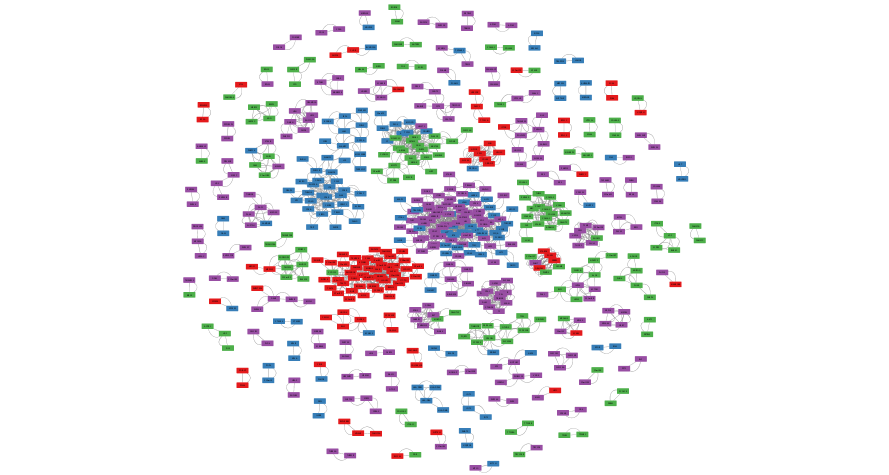
Cluster the Network
Enrichment Analysis
Enrichment Analysis - cont'd
Run g:Profiler. g:Profiler will return a set of pathways and functions that are found to be enriched in our query set of genes.
  current_cluster <- "1"
  #select all the nodes in cluster 1
  selectednodes <- selectNodes(current_cluster, by.col="__mclCluster")

  #create a subnetwork with cluster 1
  subnetwork_suid <- createSubnetwork(nodes="selected")

  renameNetwork("Cluster1_Subnetwork", network=as.numeric(subnetwork_suid))

  subnetwork_node_table <- getTableColumns(table= "node",network = as.numeric(subnetwork_suid))

  em_results <- runGprofiler(subnetwork_node_table$name)

 #write out the g:Profiler results
 em_results_filename <-file.path(getwd(),
                            "230_Isserlin_RCy3_intro", "data",paste("gprofiler_cluster",current_cluster,"enr_results.txt",sep="_"))

  write.table(em_results,em_results_filename,col.name=TRUE,sep="\t",row.names=FALSE,quote=FALSE)


  head(em_results)
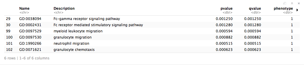
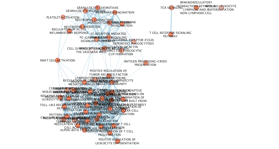
Enrichment Analysis - cont'd
Enrichment Analysis - cont'd
Export image of resulting Enrichment map.
cluster1em_png_file_name <- file.path(getwd(),"230_Isserlin_RCy3_intro", "images","cluster1em.png")
if(file.exists(cluster1em_png_file_name)){
  #cytoscape hangs waiting for user response if file already exists.  Remove it first
  file.remove(cluster1em_png_file_name)
  }

#export the network
exportImage(cluster1em_png_file_name, type = "png")
Enrichment Analysis - cont'd
Enrichment Analysis - cont'd
Export image of resulting Annotated Enrichment map.
cluster1em_annot_png_file_name <- file.path(getwd(),"230_Isserlin_RCy3_intro", "images","cluster1em_annot.png")
if(file.exists(cluster1em_annot_png_file_name)){
  #cytoscape hangs waiting for user response if file already exists.  Remove it first
  file.remove(cluster1em_annot_png_file_name)
  }

#export the network
exportImage(cluster1em_annot_png_file_name, type = "png")
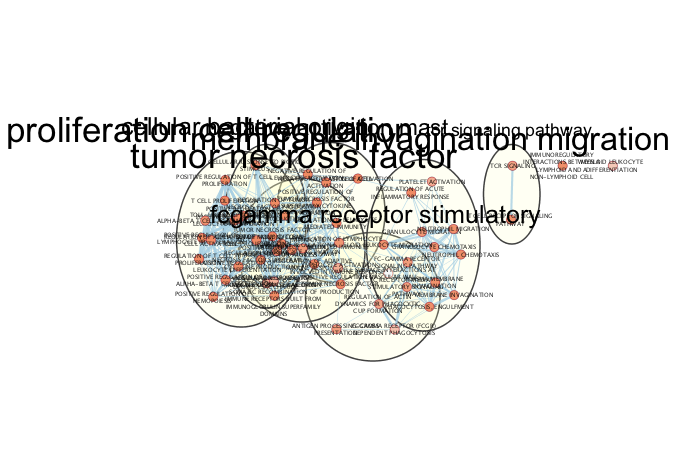
Enrichment Analysis - cont'd
Dense networks small or large never look like network figures we so often see in journals. A lot of manual tweaking, reorganization and optimization is involved in getting that perfect figure ready network. The above network is what the network starts as. The below figure is what it can look like after a few minutes of manual reorganiazation. (individual clusters were selected from the auto annotate panel and separated from other clusters)
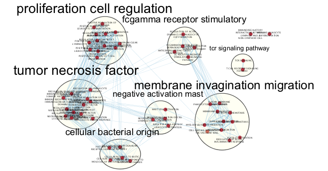
Use Case 3 - Functional Enrichment of Omics set.
Geneset Files
Geneset Files - cont'd
Geneset Files - cont'd
EnrichmentBrowser
EnrichmentBrowser - cont'd
EnrichmentBrowser - cont'd
Run basic Over representation analysis (ORA) using our ranked genes and our gene set file downloaded from the Baderlab genesets.
ora.all <- sbea(method="ora", se=se_OV, gs=baderlab.gs, perm=0, alpha=0.05)
gsRanking(ora.all)
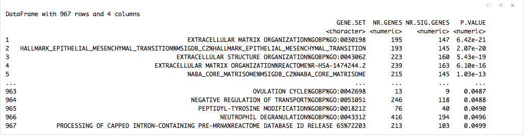
EnrichmentBrowser - cont'd
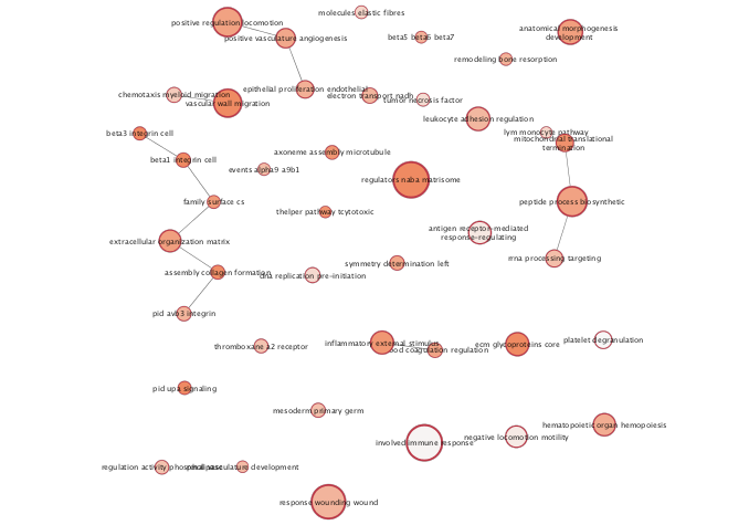
Enrichment Map
Enrichment Map - cont'd
Export image of resulting Enrichment map.
mesenem_png_file_name <- file.path(getwd(),"230_Isserlin_RCy3_intro", "images","mesenem.png")
if(file.exists(mesenem_png_file_name)){
  #cytoscape hangs waiting for user response if file already exists.  Remove it first
  file.remove(mesenem_png_file_name)
  }

#export the network
exportImage(mesenem_png_file_name, type = "png")

Enrichment Map - cont'd
Enrichment Map - cont'd
Export image of resulting Summarized Annotated Enrichment map.
mesenem_summary_png_file_name <- file.path(getwd(),"230_Isserlin_RCy3_intro","images","mesenem_summary_network.png")
if(file.exists(mesenem_summary_png_file_name)){
  #cytoscape hangs waiting for user response if file already exists.  Remove it first
  file.remove(mesenem_summary_png_file_name)
  }

#export the network
exportImage(mesenem_summary_png_file_name, type = "png")
References
Aranda, Bruno, Hagen Blankenburg, Samuel Kerrien, Fiona SL Brinkman, Arnaud Ceol, Emilie Chautard, Jose M Dana, et al. 2011. “PSICQUIC and Psiscore: Accessing and Scoring Molecular Interactions.” Nature Methods 8 (7). Nature Publishing Group: 528.
Colaprico, A., T. C. Silva, C. Olsen, L. Garofano, C. Cava, D. Garolini, T. S. Sabedot, et al. 2016. “TCGAbiolinks: An R/Bioconductor Package for Integrative Analysis of Tcga Data.” Journal Article. Nucleic Acids Res 44 (8): e71. doi:10.1093/nar/gkv1507.
Demir, Emek, Michael P Cary, Suzanne Paley, Ken Fukuda, Christian Lemer, Imre Vastrik, Guanming Wu, et al. 2010. “The Biopax Community Standard for Pathway Data Sharing.” Nature Biotechnology 28 (9). Nature Publishing Group: 935.
Grossman, R. L., A. P. Heath, V. Ferretti, H. E. Varmus, D. R. Lowy, W. A. Kibbe, and L. M. Staudt. 2016. “Toward a Shared Vision for Cancer Genomic Data.” Journal Article. N Engl J Med 375 (12): 1109–12. doi:10.1056/NEJMp1607591.
International Cancer Genome, Consortium, T. J. Hudson, W. Anderson, A. Artez, A. D. Barker, C. Bell, R. R. Bernabe, et al. 2010. “International Network of Cancer Genome Projects.” Journal Article. Nature 464 (7291): 993–8. doi:10.1038/nature08987.
Kucera, Mike, Ruth Isserlin, Arkady Arkhangorodsky, and Gary D Bader. 2016. “AutoAnnotate: A Cytoscape App for Summarizing Networks with Semantic Annotations.” F1000Research 5. Faculty of 1000 Ltd.
Langfelder, Peter, and Steve Horvath. 2008. “WGCNA: An R Package for Weighted Correlation Network Analysis.” BMC Bioinformatics 9 (1). BioMed Central: 559.
Li, B., and C. N. Dewey. 2011. “RSEM: Accurate Transcript Quantification from Rna-Seq Data with or Without a Reference Genome.” Journal Article. BMC Bioinformatics 12: 323. doi:10.1186/1471-2105-12-323.
Luna, Augustin, Özgün Babur, Bülent Arman Aksoy, Emek Demir, and Chris Sander. 2015. “PaxtoolsR: Pathway Analysis in R Using Pathway Commons.” Bioinformatics 32 (8). Oxford University Press: 1262–4.
Merico, Daniele, Ruth Isserlin, Oliver Stueker, Andrew Emili, and Gary D Bader. 2010. “Enrichment Map: A Network-Based Method for Gene-Set Enrichment Visualization and Interpretation.” PloS One 5 (11). Public Library of Science: e13984.
Morris, John H, Leonard Apeltsin, Aaron M Newman, Jan Baumbach, Tobias Wittkop, Gang Su, Gary D Bader, and Thomas E Ferrin. 2011. “ClusterMaker: A Multi-Algorithm Clustering Plugin for Cytoscape.” BMC Bioinformatics 12 (1). BioMed Central: 436.
Mostafavi, Sara, Debajyoti Ray, David Warde-Farley, Chris Grouios, and Quaid Morris. 2008. “GeneMANIA: A Real-Time Multiple Association Network Integration Algorithm for Predicting Gene Function.” Genome Biology 9 (1). BioMed Central: S4.
Oesper, Layla, Daniele Merico, Ruth Isserlin, and Gary D Bader. 2011. “WordCloud: A Cytoscape Plugin to Create a Visual Semantic Summary of Networks.” Source Code for Biology and Medicine 6 (1). BioMed Central: 7.
Ono, Keiichiro, Tanja Muetze, Georgi Kolishovski, Paul Shannon, and Barry Demchak. 2015. “CyREST: Turbocharging Cytoscape Access for External Tools via a Restful Api.” F1000Research 4. Faculty of 1000 Ltd.
Pratt, Dexter, Jing Chen, Rudolf Pillich, Vladimir Rynkov, Aaron Gary, Barry Demchak, and Trey Ideker. 2017. “NDEx 2.0: A Clearinghouse for Research on Cancer Pathways.” Cancer Research 77 (21). AACR: e58–e61.
Reimand, Jüri, Tambet Arak, Priit Adler, Liis Kolberg, Sulev Reisberg, Hedi Peterson, and Jaak Vilo. 2016. “G: Profiler—a Web Server for Functional Interpretation of Gene Lists (2016 Update).” Nucleic Acids Research 44 (W1). Oxford University Press: W83–W89.
Robinson, M. D., D. J. McCarthy, and G. K. Smyth. 2010. “EdgeR: A Bioconductor Package for Differential Expression Analysis of Digital Gene Expression Data.” Journal Article. Bioinformatics 26 (1): 139–40. doi:10.1093/bioinformatics/btp616.
Shannon, Paul, Andrew Markiel, Owen Ozier, Nitin S Baliga, Jonathan T Wang, Daniel Ramage, Nada Amin, Benno Schwikowski, and Trey Ideker. 2003. “Cytoscape: A Software Environment for Integrated Models of Biomolecular Interaction Networks.” Genome Research 13 (11). Cold Spring Harbor Lab: 2498–2504.
Szklarczyk, Damian, John H Morris, Helen Cook, Michael Kuhn, Stefan Wyder, Milan Simonovic, Alberto Santos, et al. 2016. “The String Database in 2017: Quality-Controlled Protein–protein Association Networks, Made Broadly Accessible.” Nucleic Acids Research. Oxford University Press, gkw937.
Verhaak, R. G., P. Tamayo, J. Y. Yang, D. Hubbard, H. Zhang, C. J. Creighton, S. Fereday, et al. 2013. “Prognostically Relevant Gene Signatures of High-Grade Serous Ovarian Carcinoma.” Journal Article. J Clin Invest 123 (1): 517–25. doi:10.1172/JCI65833.
Wang, K., D. Singh, Z. Zeng, S. J. Coleman, Y. Huang, G. L. Savich, X. He, et al. 2010. “MapSplice: Accurate Mapping of Rna-Seq Reads for Splice Junction Discovery.” Journal Article. Nucleic Acids Res 38 (18): e178. doi:10.1093/nar/gkq622.